Modelling with differential equations (ODE's) and parameter fitting
using the Excel® Solver

Most interesting logistic growth curves are often used for the description of bacteria dynamics. In ideal conditions with the perfect agar plate a unicellular population follows the pattern a logistic growth curve (adaption, exponential growth, stagnation at maximum) for a short period of time. In fact, those perfect dynamics vanish with the slightest change in temperature, and is not repeatable with the logistic model. Additionally, after that short static period at maximum, the population decreases again by self-inhibitory processes, followed by a rapid death period. A process which is also not covered by the basic model. 3rd. point: bacteria populations or more precise the first measurements are already in the range of >10⁴ cells per unit, means, the curvature of the lag-phase is numerically presentable by parameters with retarding effects.

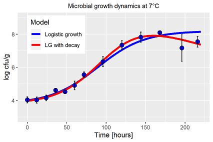
Extended conclusions of the underlying bacteria population are part of the model fitting, for example specify the population by the parameter vector with respect to the research focus. Therefore it is essential to cover the complete dynamics by the model, not only that short part, which apparently follows the pattern of the logistic curve. Even in our own work about bacteria growth on minced meat with respect to temperature (in German only) we never fulfilled those criteria (fig. 1, blue line). The significant deviance of the two last measurements have been ignored, seen as inevitable due to experimental errors. In fact, anticipating the following examples, the population has been exceeded its maximum at 7°C, first decay processes have been initiated (fig. 1, red line). To take into account the decrease, alternative models are required, the classical growth models cannot cope with decay. Why bother? As a result, the inadequacy of the Verhulst equation yields in a different estimate of the growth rate parameter r, additionally the two last measurements have affected the capacity parameter K, and lastly do not forget the high parameter correlation of those functions. All factors affect the characterization of the population by the estimated parameter vector.

In relation to the data source ¹ we calculate with cells per unit or volume, being totally aware that CCFU/ml or TVC/ml or /g are more appropriate units. Furthermore we do not refer to logarithm of the calculation, means, equations and graphics are describing the logarithm of the population size.

Also for the introduced modelling problem analytical solved solutions are available, which describe both, the sigmoidal growth plus a decreasing phase. Richter et al.² propose a function (eq. 1) with embedded switch function, which describes an exponential decrease with suitable parameter choices.

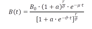
The model is well fittable to the bacteria data (fig. 1), R² ≈ 0.96, exponential growth, stagnation and senescence are repeated very well, but with given initial population the observed lag phase is not repeatable, or in other words, the fitting algorithm does not find a solution for that specific period of that data set.

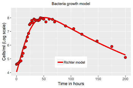
Less elegant, but more engineer like and doing its job: Replacing the capacity term of the classical growth functions (Verhulst, Richards or a modified logistic function with lag term) by an exponential decay term. The requirement is a suitable initial value at time t=0. With respect to bacteria data, the capacity can be determined in advanced, as the physical boundary of a population might be in range of about 10¹⁰ to 10¹² per volume unit (ml). The mathematical equations of fig. 2 are not represented here again.

All three models fit the data more or less well (fig. 3). While both, the Verhulst and the Richards equation, are not able to repeat the lag phase of size log 4, the third equation repeats the lag and exponential phase nearly perfect, but the period around maximum and the decay period have been fitted worse. The senescence period in fact in repeated wrongly, the residuals at that period indicate a systematic error. As the model has the highest R² value, due to better fits in certain periods with higher data densities, nevertheless, just a short period of the growth dynamic is presented well by the model.

It appears current models are lacking of precision in modelling the dynamics of all phases of bacteria populations. Leaving the analytical models and tend to numerical solved models. Based on the data set available an extension of the logistic growth curve including two switch functions is developed. The start of the exponential period is explicit switched on, and will be switched of until a critical time has passed. The first switch takes into a account the lag phase, the second switch finally initiates the decay or senescence phase (eq. 2).

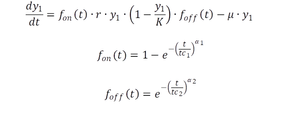
The advantage of the switch function is obvious: first the adaption period is addressed, before growth with the determined rate r starts. Means, the exponential phase starts when time approaches the critical value tc₁. Vice versa, if time approaches the critical value tc₂ growth stops, and the decay parameter μ becomes dominant and the population decreases/dies. The retarding term (1-y₁/K) is negligible in theory, but has been maintained addressing the related time related pattern in the data.

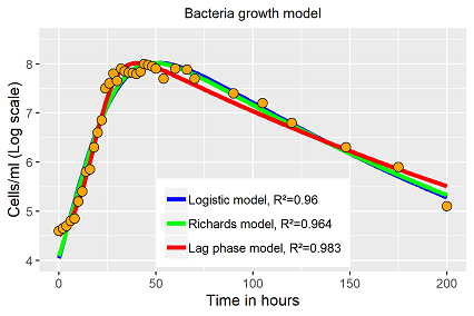
In case the video demonstration fails, fig. 4 demonstrates the fitting result of the ODE (eq. 2)

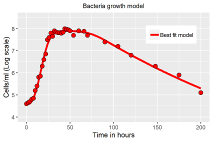
Despite the fitting appears nearly perfect (fig. 4), it has to be mentioned, the solution is not unique for this model (as so often), worse, it might depend on the initial values chosen. The underlying model includes several options: the transitions of the switch functions are smooth, if a small exponent (~2) is chosen, but sharp and sudden with higher numbers (~35). Both result in solutions with similar precision (R²>0.99), but finally in different parameter vectors. The circumstances has to be kept in mind for the comparison of different bacteria populations.

Literature:
¹Data taken from Rathmann (2012), Parameterschätzung in gewöhnlichen Differentialgleichungen, SAXSIM 2012;
²Richter & Söndgerath (1990), Parameter estimation in ecology, VCH Weinheim, 218 pp.