Modelling with differential equations (ODE's) and parameter fitting
using the
Excel® Solver
Example: Yellow rust (Puccinia striiformis) dynamics on the flag leaf of winter wheat
Summary: Based on available measurement data of yellow rust dynamics, a related ODE system is introduced and the parameter estimation problem is solved by using Excel® and the implemented Solver
The following host-parasite model is based on on personally supplied data 1 of 1997 ish, fascinating measurements, which will never show up in publications in their nativeness. As part of this parameter estimation study it offers both, the ideal opportunity to appreciate this data set and second to demonstrate the performance of the procedures introduced in this project.
On the former basis of the introduced bacteria models, similar dynamics are noticed by green canopies of annual ( and biennial) crops. An initial period of slow development is followed by an exponential expansion of the green canopy, exceeding the maximum, the canopy decreases again, concluding its life cycle by a rapid senescence pattern. This data set does not handle whole canopies, but the dynamics of the flag leaf of winter wheat. Due to the similar pattern, the dynamics of the flag leaf without yellow rust can be modelled by analytical solvable ODE's, but it does not work by integrating a fungi infection. (But is is possible to assemble model components in Excel, which allow an approximation of that problem). By this reason, only a numerically solvable solution of the ODE system to model the yellow rust experiment is introduced (eq. 1-4):
Model description
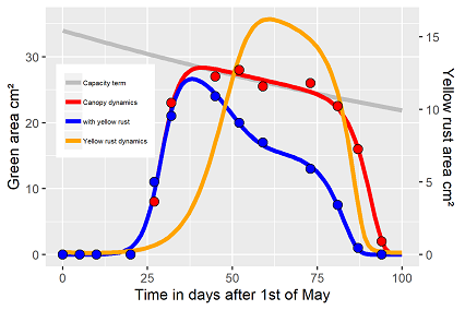
Similar to the bacteria model a time varying capacity term is introduced for a start, covering the decrease of green biomass (y1). ODE 2, y2 simulates the dynamics of the green biomass of the healthy flag leaf based on the logistic growth curve. The leaf is growing or expanding exponential with rate r. Growth/Expansion is limited by the retarding term, which decreases with the rate γ of Eq. 1. When the biological time of the flag leaf has passed, the rapid senescence is initiated by the already known type of switch function, the leaf dies with the rate μ. The model repeat the dynamics of the flag leaf with a sufficient accuracy (fig. 1). The basic model has been extended by the dynamics of the rust by eq. 3, i.e. y3. The capacity term of the leaf is additionally reduced with the rate γr. Contemporary the fungi y4grows exponential with the rate γr of eq. 4, but limited by amount of available green tissue of the flag leaf (plus a constant c. All processes finish with the death of the leaf.
The introduced model system fits the data quite well for a given set of initial values (fig. 1), indicating a certain plausibility about the assumption made during model development. The arbitrary variable ODE 1 is also depicted in fig. 1 (grey line). The resulting dynamics of P. striiformis is just speculative (fig. 1, orange line), reflecting only the assumptions made during model development. The same accounts for the chosen unit and range of the secondary y-axis. 2nd Y-axis description could be amount of mycel or numbers of uredo spores as well.
The numbers of iterations needed by the Solver indicate a certain demand and challenge of calculations. The fitting algorithm is able to identify a certain complexity and is able to repeat the data pattern.

| Table 1: Resulting parameter vectors for the ODE system | |||
|---|---|---|---|
| Solution for | Fig. 1 | Fig. 2 | Fig. 3 |
| y0 for ODE 2 and 3 | 0.000716 | 0.000711 | 0.000279 |
| r | 0.365 | 0.366 | 0.402 |
| K0 for ODE 1 | 34 | 34 | 34 |
| γ | 0.004391 | 0.004667 | 0.004575 |
| tc1 | 103.3 | 96.04 | 96.3 |
| α1 | 20.06 | 36.6 | 33.43 |
| tc2 | 97.44 | 88.2 | 92.1 |
| α2 | 15.34 | 36.40 | 35.13 |
| μ | 7.06 | 10.3 | 8.29 |
| γr | 0.633 | 0.759 | 6.697 |
| y4 (t=0) | 0.159 | 0.229 | 0.645 |
| rr | 0.1589 | 0.1413 | 0.0418 |
It has to be admitted and it is shown in table 1, again, there is no unique parameter vector, but especially the values of the switch function vary with the initial values. (tab. 1). The model concept includes several options : the switch function account for a smooth transition with small to moderate exponents (~15) or a steep transition with high exponents (~35). Larger values rarely have any further effect. Both options result in solution of similar precision. The required predetermination is also needed due to the high correlation of the two switch function parameters, and consequently affect also the critical times parameters (tc.) for the given example. The fitting procedure with small exponents as initial values resulted with tc-values of 103 days (of the given time scale), and 98 respectively, beyond the measurement time range. For the large exponents tc-values of 96 and 88 day have been the result (fig. 3). The fitting precision of fig. 3 seems to be a tiny bit poorer, but the tc-values end up in the observed time ranges. Again, the problem is crucial, if statistical comparisons are the purpose of the modelling approach, hence use one common set of initial values for all factor levels.
Ignoring the question or concerns about the exact parameter estimates, the conclusions of this experiment are obvious. The active photosynthetically capacity is not only significantly reduced, but the longevity of the flag leaf is noticeable shortened. Both dependencies are quantified by the parameters. The relative difference of the tc-values specifies the numbers of days lost for photosynthesis, the even more fascinating parameter γr describes not only the intensity of additional losses in green biomass, therefore could be a measure of the pathogenicity of the fungi, but also a measure of the resistance of the host variety. These parameters are quantitative comparable in further, similar experiments by the use of such ODE systems with estimated parameters, if data of different P. striiformis strains are available or such experiments are performed with different varieties. Further result of the parameter fitting: the dynamics of yellow rust are the simulated result of the model only, no related data have been available. But as a result of the parameter fitting, both estimates of the initial value y4 (t=0) and the growth rate parameter rr were found to be relatively large.
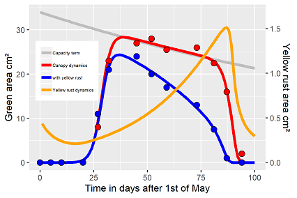
Most interesting an alternative initial value vector yielded another, a little bit unexpected and not fully explainable Solver solution (fig. 3). Most frankly, the first reaction, especially the simulated rust dynamics, has been directly and as not plausible declined. Firstly, the curvature of the infected flag leaf has been apparently ignored, but does it exist in that way of the previous fits? 2nd the Solver fit resulted in initial values of the yellow rust twice that high as before. An initial decline is recorded, as no flag leaf has emerged yet. With passing time the fungi attacks the expanding and fresh flag leaf with high sporulation, rust growth accelerates with green tissue availability as long as the fungi population collapses with the dying flag leaf. But the maximum values are in the range of 2.5 (fig3), not 14 to 16 cm2 as before (fig 1, 2). The result is feasible. During the vegetation period Yellow rust jumps by sporulation from leaf layer to leaf layer. The existence of a high sporulation potential before flag leaf emergence is therefore explainable from the biological point of view. The resulting parameter vector describes a different yellow rust dynamic as the two earlier fits. Which of the solutions is the "right" or "best". This question cannot be cleared without related P. striiformis data.
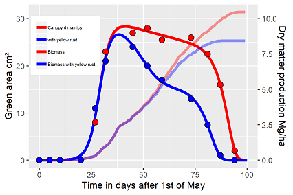
Finally, what are the implications of this yellow rust infestation? As the flag leaf contributes to yield by 95%, it is the task of any canopy management to keep the flag leaf alive as long as possible. Based on a Beer's Law approach for light interception and available radiation data of that year the following dry matter production rates have been simulated (fig. 4). The trajectories are not presenting yield, but simple the C-accumulation based on the photosynthetically activity. Fig. 4 demonstrates the light induced growth rate is changing when the flag leaf has lost about 25% its green tissue, around day 55. Finally the C-losses are in the range 12% by the yellow rust reduced area of photosynthesis and additional 8% are caused by the reduced longevity of 6-8 days of the flag leaf.
Resume
Well known problems with such models, there is no unique solution for such systems. Especially if part of the system are not verified by data. The Solver algorithm offers by the simultaneous parameter estimations die opportunity to limit die choice of solutions. It remains important, as mentioned before, using such models as regressions functions for the analysis of field- and lab trials require the common use of the same initial values for all factor levels to address differences of the parameter vectors according to the related factor level. The problem of the time switch parameter has been discussed before.
Literature:
Use of in-field measurements of green leaf area and incident radiation to estimate the effects of yellow rust epidemics on the yield of winter wheat
(1997) R.J. Bryson et al., https://doi.org/10.1016/S0378-519X(97)80010-4

