Home Models Consulting News Order

Example: temperature driven growth dynamics of melon seedlings.

Summary: Based on example data of the growth of melon seedlings at different constant temperature levels an ODE model is introduced, commonly covering experiments with several factor levels. The example describes the plant growth pattern at temperature levels from 25°C to 37.5°C, parameter estimation of different types of model, which have been tested with respect to the underlying data, has been performed with the Solver. While the models introduced before have been covering the horizontal regression problem (with time), the extension of this chapter is dealing with the vertical regression problem, covering different factor levels, temperature levels, etc. Focus is the comparison of two step fitting procedures versus simultaneous fitting of all factor levels.

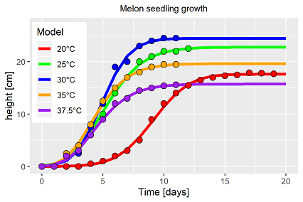
The growth model is based on the data of melon seedlings, grwon at different constant temperature levels (Pearl et al., 1934, data taken from "Models in Biology", 1994)¹. While Brown & Rothery demonstrated only the fitting possibility of different type of the Richards function, the data structure offers much more complexity including much more interesting challenges. In short, the data can be summarised to: growth rate as well as plant height vary with temperature, not surprising. But, temperature levels range far into supra-optimal degrees (fig. 1).

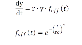
To model the basic dynamics a simple nonlinear ODE growth model with a switch off function is introduced (eq. 1). In words, the plant grow with the rate r until time t approaches and exceeds the critical time tc.

Case 1: Parameter estimation of a two stage procedure

Eq. 1 has been separately fitted to the data of each temperature level as an initial step. Fig. 1 demonstrates the result graphically. Eq. 1 is commonly applicable, the fits resulted in an individual parameter vector for each temperature level (table 1). Contrary to the conclusions of Brown & Rothery (1994)¹ the introduced model fits the data with sufficient precision (R²>0.99), fig. 1.

Table 1 presents the estimators, but initial values and the form parameter α has been set constant for all temperature levels.

Table. 1: resulting estimates of the ODE model
Parameter	20°C	25°C;	30°C	35°C	37,5°C
r	0.81	1.48	1.59	1.70	1.55
tc	8.28	4.63	4.39	3.95	4.15

Parameter r (for growth) and 1/tc (for development) are fitted to related temperature response functions in the second analysis step. Usually, the O'Neill function is used. Due to its complexity and numerous repetition on this web site we refer to a related report, page 2 . Four parameter to estimate (r_max, Q10, Topt & Tmax) and 5 measurements (=primary parameter taken from the first fit) fulfill just the statistical basics.

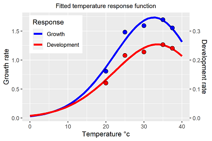
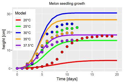
Fig. 2 shows graphically the fits to the chosen temperature response function. The O'Neill function is suitable to functionalize the biological impact of temperature. Please notice the different scales of the y-axeses in fig. 2. In theory, this estimated response function represents the common parameter vector for all temperature levels. To validate the findings so far, setting the estimated rate and development parameters back into the basic model ended up with the trajectories shown in figure 3. The results demonstrate more than obvious the failure of this strategy.
Hence, an alternative solution is introduced.

Case 2: Analysing all temperature levels by simultaneous parameter estimation

Introducing the topic of simultaneous parameter estimation two additional basics are presented: Eq. 2 introduces the minimising problem to solve:

with a=5 temperature levels available, and n_i the number of measurements at temperature level i. The residual sum of squares are minimised with respect to the data j of temperature level i and the function values at time t_i,i with given parameter vector θ.
The basic model is extended for the simultaneous fitting as follows: (Eq. 3):

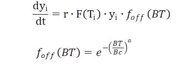
while the growth rate r times the F(T)_i is determined by the O'Neil function at temperature i. The time to switch off growth is also controlled by temperature and defines the Biological Time, bulding the sums of the fraction of the development rate of each temperature level, again based on the given temperature response function. Growth stops when the Biological Time approaches and passes the critical time point Bc.

To keep the models as parsimonious as possible, the simultaneous parameter estimation has been started with one common temperature response function for both, growth and development. Fig. 4 depicts the result. The solver approximated to that apparent "optimum", indicating false model assumptions.

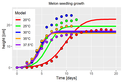
The less than poor result has not been surprising. The single fit results indicated already that growth and development respond different to changes in temperature (fig. 2). But before extending the model type it has to be tested if the Solver is able to identify an average model compared to the observations. That has not been the case. The model has been extended for each process by its own temperature response function, introducing the indices g (~growth) and d (~development). The results are shown in fig. 5 and 6.

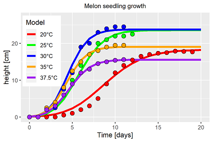
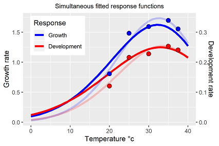
In fact, Solver is able to find a solution for the extended model, which takes into account all measurement data from five temperature level for the fitting. The resulting trajectories fits the data well (fig. 5). Temperature affects the plant dynamics ( here melon seedlings) twice with different intensity, each of the processes(growth, development) require a temperature response function of its own. Comparing the estimated parameters of the temperature response functions from eq. 3 with the single fit results (fig. 6) the differences are marginal, probably not different in statistical terms. But, due to the nested non-linearity of growth model and embedded temperature response function, the differences are massive. Table 2 summarises for several reasons the resulting parameter vector of eq. 3:

Tabelle 2: resulting parameter values of the ODE model with 2 temperature response functions
Parameter	y0	rg	Q10g	Toptg	Tmaxg	rd	Q10d	Toptd	Tmaxd	Bc	α
Estimates	0.1	1.625	1.949	32.284	89.335	1.054	1.832	33.018	100.0	4.536	2.003

• The initial values y_0,i for all temperature levels have been set.
• The estimators of table 2 present an extremely narrow parameter vector (~ perhaps some kind of "perfect" solution?)), but, tiny variation in this vector caused massive deviance in the trajectories. It indicates a certain type of instability, but, the data define the boundaries, not the underlying mathematics.
• Solver does not approximates the Tmax-values. The given, very large boundary values have been approached by the algorithm. But, in case of choosing smaller boundary values, the whole model does not approximate, means, even the unrealistic Tmax values have their reasons.
• The simultaneous fitting of non-linear systems has to be seen superior with respect to result and information value compared to the two stage procedure, especially if transferable knowledge should identified and analysed.
• The use of Solver gains precisions of the parameter estimates, which are much more meaningful than any hand fitting techniques.
• The question about the temperature optimum is answered much more precise by the procedures introduced here.

Resume

A simple data set, ancient, even trivial, extremely challenging. It is in fact of no interest, if the original authors have been truly able to maintain constant temperatures throughout the experiment. Even nowadays somewhat tricky. No problem at all. The result includes the real, but unknown temperature pattern of the 1934 trials. In the beginning of this exercise it was not clear whether satisfying results would be achievable, which would be worth to be taken into account in this chapter about parameter estimation in ODEs. The data including the analysis procedure offers a potential solution about the relevant question in canopy dynamics, how much is growth, how much is development. Without stressing the interpretation too much, the analysis procedures demonstrate furthermore the possibility, how the iterative technique of working hypothesis, model links and Solver solutions (or similar methods in Matlab, Python, etc.) can be performed until plausible results are achieved (if there are any). Summarising the tested model combinations revealed different response functions for the same data set. Minor differences are caused by the fitting procedure, but a single consideration of the identified temperature response function is not feasible for any application, as the parameters changes with the underlying model. As shown in this example, nested non linear processes must be seen as an inseparably unit. Hence, using such temperature response functions in a predictive mode, the underlying model has to be taken into account as well. Both, the growth model and the temperature response function must be seen as one unit for any application.

Literatur:
¹Models in Biology, Mathematics, Statistics and Computing, D. Brown & P. Rothery, (1994), Seite 50.